Reinforcement Learning
Florian Lüscher
Reinforcement Learning is a hot topic right now. Especially after the successes of AlphaGo and it’s extensive media coverage. But reinforcement learning is capable of much more than playing computer games, even though the videos are awesome to watch. Different companies are investing heavily into research of the field.
What is Reinforcement Learning?
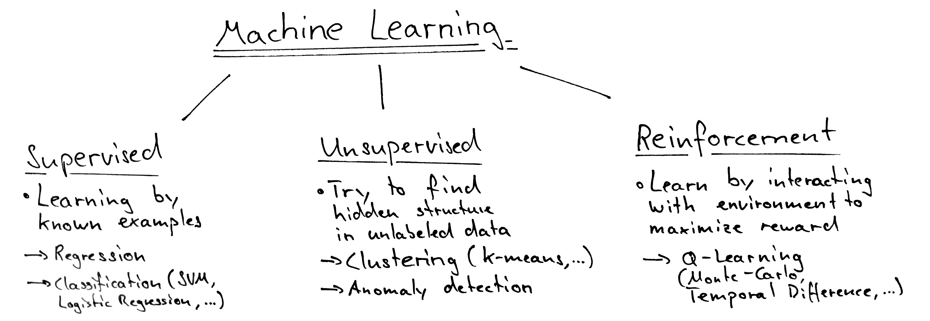
You probably already know that there are different possiblities to train a Machine Learning model. You might have heard of linear models like linear regression or other algorithms like k-means clustering. These algorithms are usually divided into two categories: supervised and unsupervised learning. So where does reinforcement learning fit in? As it turns out, reinforcement learning doesn’t quite fit into any of the two categories and is therefore often considered a third one all by itself.
When we use supervised learning to train a model, we already have a set of examples for which we know the expected answers. When using unsupervised learning, we only have the data, but don’t know the “labels” of this data. So what does reinforcement learning do differently? In Reinforcement Learning, an agent learns by interacting with it’s environment and triyng to maximize some sort of long-term reward.
So while we need data and labels in the case of supervised and unsupervised learning, we don’t need that when doing reinforcement learning. But we need to provide the algorithm the means to observe and modify it’s environment. When learning, we let the agent modify it’s environment by performing some sort of action and tell him how much reward it earned by doing so. This of course works well for computer games, since we already have the environment (the game itself), the possible actions (the possible inputs of the player) and a method to calculate the reward (the score in the game). But you can imagine that this is a bit more complicated when the agent interacts with the real world (a robot in a room).
Components of Reinforcement Learning
When training a model using reinforcement learning, there are four components involved:
-
A Policy is the core of a reinforcement learning algorithm. It is a function mapping a given state to the next action to perform. While learning the agent changes his policy in order to maximise the reward.
-
The Reward Function defines the reward a agent can expect at given a state/timestep. Since this is the function the agent tries to maximise, it is unmodifiable during training.
-
A Value Function is an estimation about how much reward an agent can expect when entering specific state. It is different from the reward function in that the reward is definitive and immediate, whereas the value is predicted and therefore unsure.
-
A Model of the environment can help the agent in planning it’s future moves. A model might be made available to the agent because it was provided by the developer or a model might be learned during training.
This for sure sounds confusing. So probably it’s best to just jump to an example of this.
Example: Tic-Tac-Toe
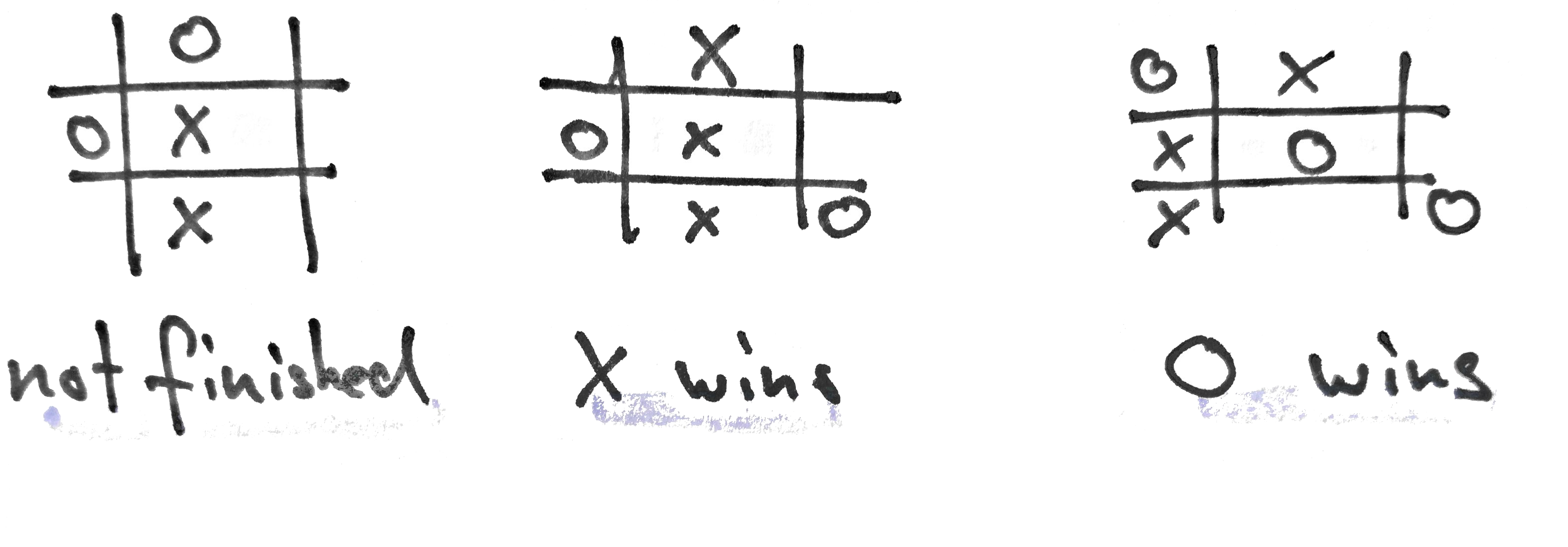
Since reinforcement learning components map good to games we try to explore the concept by writing an AI-player for the simple game of Tic-Tac-Toe. The game is extremely simple: Two players (X and O) play one after another by marking a field. As soon as one player has three fields in a row, column or diagonally, he wins. If all fields were marked, the game is a draw.
Our Model
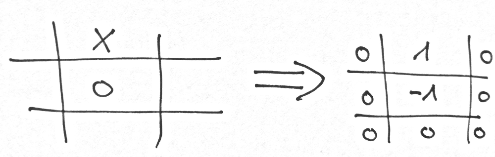
So first, we are going to implement our model. Since the game is that simple, our model is too. We can map the field of the game to a simple array. This means every field now has a fixed number (the index in the array). Furthermore we use three numbers to determine the value of a field (0 = unoccupied, 1 = occupied by agent, -1 = occupied by opponent).
If we implement this model in Python it might look something like this:
AGENT = 1
OPPONENT = -1
NO_PLAYER = 0

class Game:
    def __init__(self, game_state=None):
        if game_state is None:
            game_state = [
                0, 0, 0,
                0, 0, 0,
                0, 0, 0
            ]
        self.state = game_state

    def __str__(self):
        return str(self.state)

    def is_draw(self): pass
    def is_finished(self): pass

    def valid_moves(self): pass
        # returns list of fields which are unoccupied
    def make_move(self, field, player): pass
        # marks field as occupied by player
    def get_winner(self): pass
        # Returns the winner [-1 or 1] or 0 if draw
The implementations are left out for readability. Now that we have our model it’s time to think about the simplest possible policy: the random policy takes a random action from all possible moves:
import random

def random_policy(game):
    return random.choice(game.valid_moves())
So given that policy, we can let two random policies play against each other!
def play_games(policy, opponent_policy, num_games=100):
    games_won = 0
    draw = 0
    # Play games
    for i in range(num_games):
        game = Game()
        # 50% chance opponent starts
        if random.random() > 0.5:
            game = game.make_move(opponent_policy(game), OPPONENT)

        while not game.is_finished():
            # First players turn
            game = game.make_move(policy(game), AGENT)
            if game.is_finished():
                break
            # Other players turn
            game = game.make_move(opponent_policy(game), OPPONENT)

        if game.get_winner() == 0:
            draw = draw + 1
        if game.get_winner() > 0:
            games_won = games_won + 1

    return games_won, draw

games_won, draw = play_games(policy=random_policy,
                             opponent_policy=random_policy,
                             num_games=1000)
print("Games won: %s" % games_won)
print("Draw: %s" % draw)
Which of course returns a result where about half the played games are won or draw:
Games won: 432
Draw: 129
We can for sure do better than that! In fact, we haven’t learnt anything so far. But what should we learn?
A Tabular Value Function
Remember that we only used two of the components of Reinforcement Learning so far: the policy and the model. So let’s talk about the other two. The reward in the case of tic tac toe is pretty simple too. You don’t get any points during the game, but if you win at the end you receive one point. Translated to our Python model a simple reward function might look like that:
def reward(game):
    return max(game.get_winner(), 0)
Now let’s have a look at one situation in the game, where our agent considers two possibible actions:
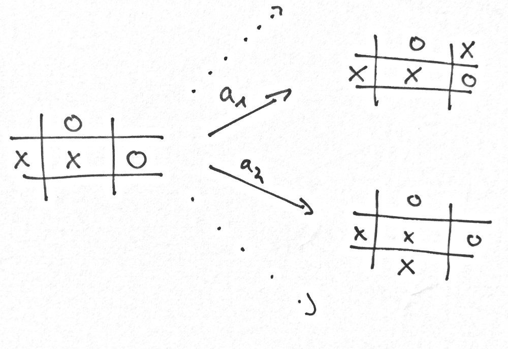
Our policy now somehow needs to decide what to do next. Because we implemented our model it can take the current state and calculate all the possible actions (a1, a2) and see to which state any action would lead. But since we are in the middle of the game, the reward function returns zero for every state. This isn’t very helpful. And this is the point where the value function comes into play. Rembember, we said the value function is a prediction about the expected reward. But where does that value come from? The simplest form of our value function is a tabular mapping from state to value:
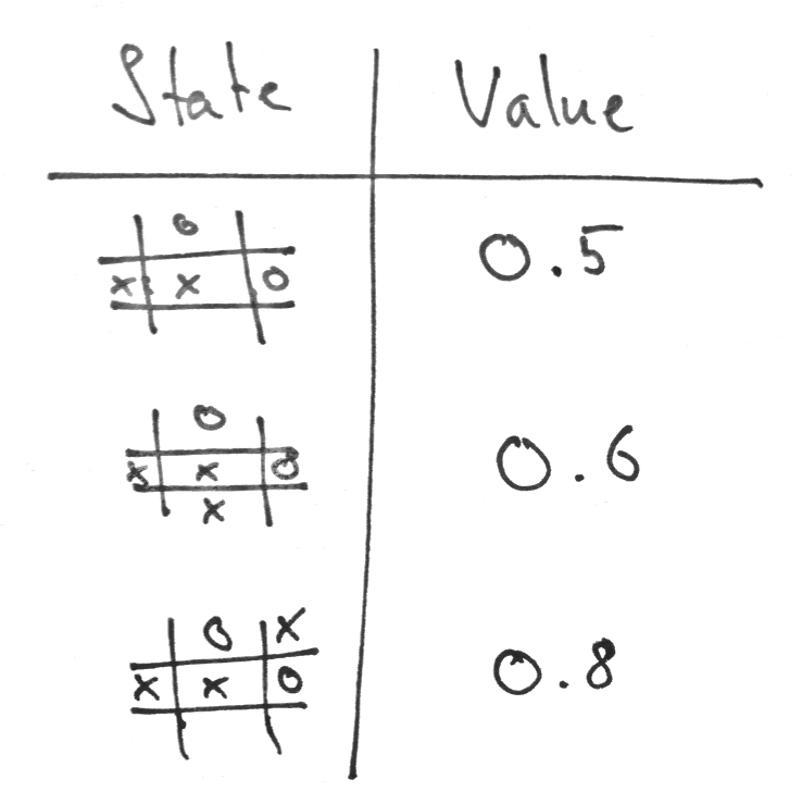
Given that value function, our policy could choose the action leading to the state with the highest possible reward. In this case a1 would lead to a state with a higher value than a2. The following Python implementation shows a policy backed by the value table values.
class ValuePolicy:
    DEFAULT_VALUE = 0.5

    def __init__(self):
        self.values = {}

    def policy(self, game):
        move_values = {}
        moves = game.valid_moves()
        for move in moves:
            next = game.make_move(move, AGENT)
            move_values[move] = self.get_state_value(next)

        return max(move_values, key=move_values.get)

    def get_state_value(self, state):
        if str(state) not in self.values:
            return self.DEFAULT_VALUE

        return self.values[str(state)]
We can use this policy to run against our random_policy and see what happens.
value_policy = ValuePolicy()
games_won, draw = play_games(policy=value_policy.policy(),
                             opponent_policy=random_policy,
                             num_games=1000)
print("Games won: %s" % games_won)
print("Draw: %s" % draw)

# Output:
# Games won: 579
# Draw: 36
Interesting, somehow this policy is better, even though our value table does not contain any value at all! This is because in this case the ValuePolicy starts filling out the field from the top left to the bottom right, which apparently is a better strategy than the random one.
Learning the Tabular Value Function
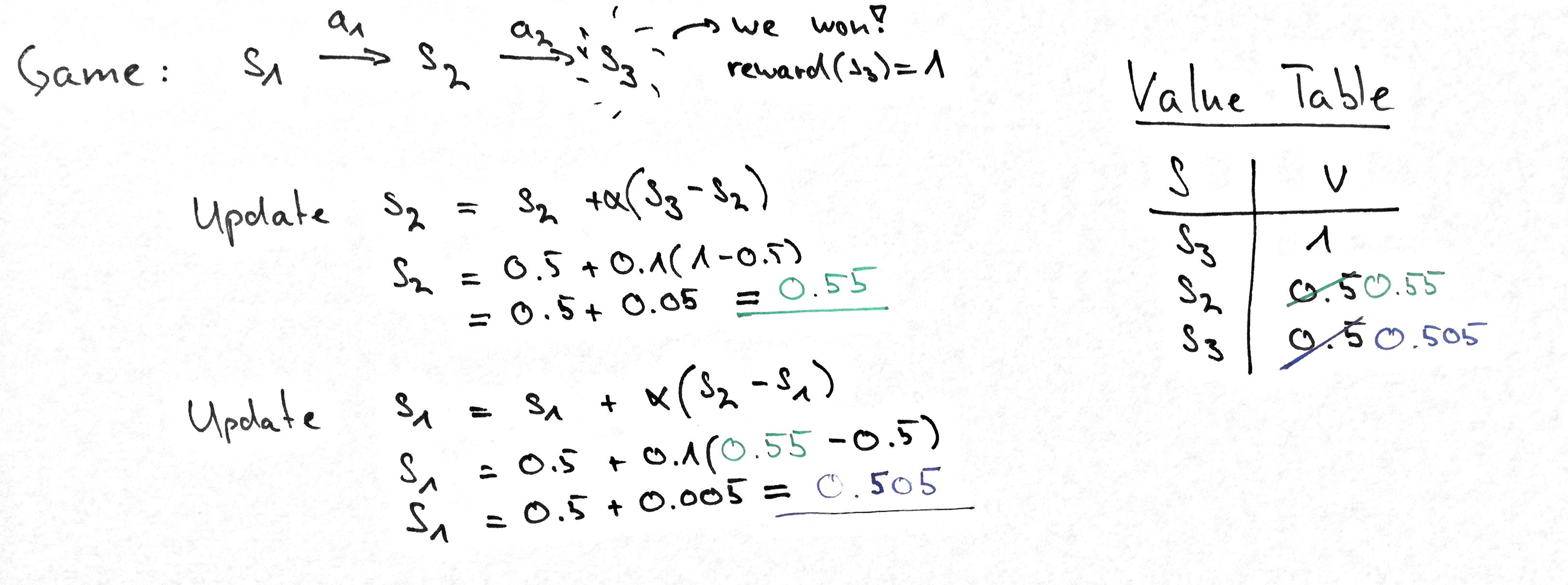
Finally we come to the most intersting part. We already have most of the components ready but you might have noticed that our program has not learned anything so far. We know that if we have values for our states in the value table, our policy would choose the action with the highest potential reward. But since our reward function only gives reward for victories at the end of each game, we need a method to pass that reward back to the earlier states. Because these states came before the end state this method is called temporal-difference learning. This learning method is based on playing a lot of games, and updating the values of every state after each game based on the reward at the end of the game. Usually the update involves a learning rate α. In our following example we use a learning rate of 0.1.
Lets have a look at how this algorithm is implemented on our ValuePolicy:
class ValuePolicy:
    DEFAULT_VALUE = 0.5

    def __init__(self):
        self.values = {}

    # Rest of class omitted

    def set_state_value(self, state, value):
        self.values[str(state)] = value

    def learn(self, states):
        # Actually perform the learning
        def temporal_difference(current_state_value, next_state_value):
            learning_rate = 0.1
            return current_state_value +
                learning_rate * (next_state_value - current_state_value)

        last_state = states[-1:][0]
        last_value = reward(last_state)
        self.set_state_value(last_state, last_value)
        # Go through every state from end to start
        for state in reversed(states[:-1]):
            value = self.get_state_value(state)
            last_value = temporal_difference(value, last_value)
            self.set_state_value(state, last_value)
So with our learning algorithm in place the only thing left to do is to simulate a lot of games and update the value table.
def train(policy, opponent_policy, training_games=1000):
    for i in range(training_games):
        game = Game()
        states = []

        # 50% chance opponent starts
        if random.random() > 0.5:
            game = game.make_move(opponent_policy(game), OPPONENT)

        while not game.is_finished():
            # Our agent makes a move
            game = game.make_move(policy.policy(game), AGENT)
            states.append(game)

            if game.is_finished():
                break

            game = game.make_move(opponent_policy(game), OPPONENT)
            states.append(game)

        policy.learn(states)

train(policy, random_policy, training_games=20000)
print(policy.values)

# Outputs:
#
# {'[1, 0, -1, -1, 0, 0, 0, 1, 0]': 0.5070510416675937, '[1, -1, -1, 1, 1, -1, 0, 1, 0]': 0.45, ...
After training you can see that we trained our tabular value function so that some states have a better value than others. And if we put that all together we can first train our model and after that run a couple of games against our random_policy:
policy = ValuePolicy()

train(policy, random_policy, training_games=20000)

games_won, draw = play_games(policy.policy, random_policy, 1000)

print("Games won: %s" % games_won)
print("Draw: %s" % draw)

# Output:
# Games won: 581
# Draw: 53
Hmm. That is not so good. Why is that? We achieved a similar score without any values in the table!
Exploration vs Exploitation
The policy we implemented is called a greedy policy, because it always chooses the action leading to the highest reward. Can you imagine what happens during training? If we always follow the best one, we don’t get to see all the other possibilities. But these unknown states might lead to the higher reward. So we somehow need to get our algorithm explore different branches. We achieve this by sometimes select a random action during training:
def train(policy, opponent_policy, training_games=1000):
    for i in range(training_games):
        game = Game()
        states = []

        # 50% chance opponent starts
        if random.random() > 0.5:
            game = game.make_move(opponent_policy(game), OPPONENT)

        while not game.is_finished():
            # Our agent makes a move
            # but occasionally we make a random choice
            if random.random() < 0.1:
                game = game.make_move(random_policy(game), AGENT)
            else:
                game = game.make_move(policy.policy(game), AGENT)
            states.append(game)

            if game.is_finished():
                break

            game = game.make_move(opponent_policy(game), OPPONENT)
            states.append(game)

        policy.learn(states)
With this change in place we achieve over 90% victory rates against the random policy:
policy = ValuePolicy()

train(policy, random_policy, training_games=20000)

games_won, draw = play_games(policy.policy, random_policy, 1000)

print("Games won: %s" % games_won)
print("Draw: %s" % draw)

# Output:
# Games won: 926
# Draw: 22
This balance between exploiting and exploring is a common difficulty in Reinforcement Learning algorithms and requires careful tuning by the developer.
Conclusion
We saw a simple temporal-difference learning algorithm in action. Reinforcement Learning can do much more than just that. Our policy and value function were the most basic ones. World-class implementations like AlphaGo use neural networks to approximate the ideal value and policy functions and combine them with a classical algorithms like Monte Carlo Tree Search .
If you are interested in the topic, I strongly recommend to have a look at the book by Richard Sutton and Andrew Barto.
If you want to experiment with the code used in this article you find it on Github. You can run the examples yourself and play directly with the code with mybinder.org.
Please don’t hesitate to contact us if you need a strong partner to successfully integrate artificial intelligence and machine learning to your business.